A Course on Numerical Linear Algebra¶

Instructor: Deniz Bilman

Textbook: Numerical Linear Algebra, by Trefethen and Bau.

Lecture 7: QR Factorization¶

The main idea of QR factorization of a given matrix $A \in\mathbb{C}^{m\times n}$ is to construct a sequence of orthonormal vectors $q_1, q_2,\ldots, q_r$, $r=\operatorname{rank}(A)$, that span the successive column spaces of $A$:

\begin{align*} \operatorname{span}(\{A_{:,1}\}) &= \operatorname{span}(\{q_1\})\\ \operatorname{span}(\{A_{:,1},A_{:,2}\}) &= \operatorname{span}(\{q_1,q_2\})\\ \operatorname{span}(\{A_{:,1},A_{:,2},A_{:,3}\}) &= \operatorname{span}(\{q_1,q_2,q_3\})\\ &\vdots \end{align*}

Thin (Reduced) QR Factorization¶

Let's focus on the case $A\in\mathbb{C}^{m\times n}$, $m\geq n$, of full rank $r=\operatorname{rank}(A)$. The goal then is to have a sequence of vectors $q_1,q_2,\ldots$ such that

$$ \operatorname{span}(\{q_1,q_2,\ldots q_j\}) = \operatorname{span}(\{A_{:,1},A_{:,2}, \ldots, A_{:,j}\}),\qquad \text{for each}\quad j=1,2,\ldots,n. $$

In terms of linear combinations of column vectors, this reads $$ \begin{bmatrix} A_{:,1} & A_{:,2} & \cdots & A_{:,n} \end{bmatrix} = \begin{bmatrix} q_1 & q_2 & \cdots & q_n \end{bmatrix} \begin{bmatrix} r_{11} & r_{12} & \cdots & r_{1 n} \\ & r_{22} & & \vdots \\ & & \ddots & \\ & & & r_{n n} \end{bmatrix} $$ for some scalars $r_{jk} \in \mathbb{C}$ with $r_{kk}\neq 0$ for $k=1,2,\ldots n$. (Exercise: Why is the diagonal nonzero?)

This factorization of $A$ yields the following equations

$$ \begin{aligned} A_{:,1} & =r_{11} q_1 \\ A_{:,2} & =r_{12} q_1+r_{22} q_2 \\ A_{:,3} & =r_{13} q_1+r_{23} q_2+r_{33} q_3 \\ & \vdots \\ A_{:,n} & =r_{1 n} q_1+r_{2 n} q_2+\cdots+r_{n n} q_n \end{aligned} $$

In terms of matrices, this reads $$ A = \hat{Q} \hat{R}, $$ where $\hat{Q}$ is an $m\times n$ matrix (the same size as $A$) with orthonormal columns and $\hat{R}$ is an $n\times n$ upper-triangular matrix with nonzero diagonal.

This factorization is called reduced QR factorization of $A$ of $A$ or reduced QR factorization of $A$.

Full QR Factorization¶

Just like in SVD (Lecture 5), we can append an additional $m-n$ orthonormal columns to $\hat{Q}$ and extend it to an $m\times m$ unitary matrix $Q$. Accordingly, we append $m-n$ zero rows to $\hat{R}$ to extend it to an $m\times n$ matrix $R$ so that the extraneous columns of $Q$ remain silent in the factorization

$$ A = Q R $$

This is called the full QR factorization of $A$.

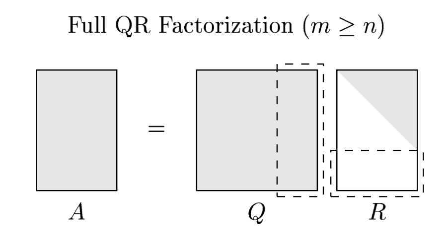
(Full QR Factorization from Trefethen & Bau.

Note that the in the full QR factoriation, the columns $q_j$ for $j>n$ are orthogonal to $\operatorname{range}(A)$. Assumin $A$ is of full rank $n$, those vectors constitute an orthonormal basis for the space $\operatorname{range}(A)^{\perp}$.

Gram-Schimdt Orthogonalization¶

The QR factorization can be constructed using the classical Gram-Schmidt orthogonalization process --- a successive orthogonalization procedure. It goes like this

Initial step: Take $A_{:,1}$, normalize it, and call it $q_1$.

Iterated step: For $j=2,3,4,\ldots$ successively, construct:

$$ v_j = A_{:,j} - (q_1^* A_{:,j}) q_1 - (q_2^* A_{:,j}) q_2 - \cdots - (q_{j-1}^* A_{:,j}) q_{j-1}, $$

normalize it, and call it $q_j$. At each stage one projects the relevant column of $A$ onto the existing orhonormal vectors $q_k$, $1\leq k\leq j-1$ and substract this projection from that column of $A$ to obtain a vector in the orthogonal complement.

So, we may rewrite the QR factorization equations in the form:

$$ \begin{aligned} q_1 & =\frac{A_{:,1}}{r_{11}}, \\ q_2 & =\frac{A_{:,2}-r_{12} q_1}{r_{22}}, \\ q_3 & =\frac{A_{:,3}-r_{13} q_1-r_{23} q_2}{r_{33}}, \\ & \vdots \\ q_n & =\frac{A_{:,n}-\displaystyle\sum_{i=1}^{n-1} r_{i n} q_i}{r_{n n}} . \end{aligned} $$

It is now clear that the scalars in the numerators are $$ r_{i j}=q_i^* A_{:,j} \quad\text{for}\quad i \neq j $$ and the coefficients $r_{i j}$ in the denominators are chosen for normalization: $$ \left|r_{j j}\right|=\left\|a_j-\sum_{i=1}^{j-1} r_{i j} q_i\right\|_2 $$

Note that the sign of $r_{j j}$ is not determined. Arbitrarily, we may choose $r_{j j}>0$. In this case we arrive at the factorization $A=\hat{Q} \hat{R}$, where $\hat{R}$ has positive entries along the diagonal.

The Gram-Schmidt orthogonalization process in the form described above (called the classical Gram-Schmidt iteration) is numerically unstable due to rounding errors on a computer. There is the modified Gram-Schmidt iteration that overcomes this issue. We will cover that later on.

Existence and Uniqueness¶

Theorem:¶

Every $A \in \mathbb{C}^{m \times n}(m \geq n)$ has a full $Q R$ factorization, hence also a reduced QR factorization.

Theorem:¶

Each $A \in \mathbb{C}^{m \times n}(m \geq n)$ of full rank has a unique reduced $Q R$ factorization $A=\hat{Q} \hat{R}$ with $r_{j j}>0$.

In [16]:

# We can implement the QR factorization using the ideas above as follows:
A = round.(10*rand(8,6))
A|>display
(m,n) = size(A)
Q = zeros(m,n)
R = zeros(n,n)

# Classical Gram-Schmidt iteration
R[1,1] = norm(A[:,1]);
Q[:,1] = A[:,1]/R[1,1];
for j = 2:n
    R[1:j-1,j] = Q[:,1:j-1]'*A[:,j];
    v = A[:,j] - Q[:,1:j-1]*R[1:j-1,j];
    R[j,j] = norm(v);
    Q[:,j] = v/R[j,j];
end

A - Q*R

8×6 Matrix{Float64}:
 8.0   2.0  1.0   2.0  9.0  8.0
 5.0   3.0  5.0  10.0  5.0  3.0
 6.0   6.0  9.0   0.0  4.0  9.0
 9.0   2.0  9.0   5.0  0.0  6.0
 6.0  10.0  8.0   7.0  1.0  3.0
 9.0   3.0  9.0   5.0  2.0  2.0
 2.0   1.0  4.0   2.0  8.0  8.0
 8.0   1.0  1.0   0.0  2.0  9.0

8×6 Matrix{Float64}:
 0.0  0.0  3.33067e-16  0.0           0.0          0.0
 0.0  0.0  0.0          0.0           0.0          0.0
 0.0  0.0  0.0          9.69058e-17   0.0          0.0
 0.0  0.0  0.0          0.0          -4.76599e-18  0.0
 0.0  0.0  0.0          0.0           0.0          0.0
 0.0  0.0  0.0          0.0           0.0          2.22045e-16
 0.0  0.0  0.0          0.0           0.0          0.0
 0.0  0.0  2.22045e-16  3.37139e-17   0.0          0.0

Solution of $Ax=b$ by QR Factorization¶

Suppose we want to solve $Ax=b$ for $x$, where $A\in\mathbb{C}^{m\times m}$ is nonsingular. If $A=QR$ is a QR factorization, then we can write

$$ Ax = b \iff QR x = b \iff R x = Q^* b. $$

When $Q$ is known, the RHS is easy to compute. $Rx = y$ is also easy to solve (by backward substitutiton) because $R$ is upper triangular. So the steps to solve $Ax=b$ using QR factorization would be:

Compute a QR factorization $A=Q R$.
Compute $y=Q^* b$.
Solve $R x=y$ for $x$.

We will present algorithms for each of these steps later in the course. This is a great method, but it requires significantly double the amount of flops compared to the Gaussian elimination.

In [9]:

using LinearAlgebra

m = 8; # dimension
A = round.(10*rand(m,m))
b = collect(1:m)

(Q,R) = qr(A)

btilde = Q'*b

8-element Vector{Float64}:
 -8.64612951299919
 -4.040288101752376
  3.384526861747502
  7.507609234337892
 -1.8135476892481837
  0.3034179084435218
  0.3389717021952645
  6.450223138980993

In [12]:

# Now implement back-substitution
x = zeros(m);
x[m] = btilde[m]/R[m,m];
for i = m-1:-1:1
    y = btilde[i] - dot(R[i, i+1:m], x[i+1:m]);
    x[i] = y[1] / R[i,i];
end
# Check the size of the residual:
norm(A*x - b)

1.0245379651382904e-14

QR Factorization as an Eigenvalue Algorithm: The QR Algorithm¶

The QR algorithm as a method to compute the eigenvalues of a square matrix dates back to 1960s. In its simplest form, it goes like this:

\begin{align*} &A^{(0)}:=A\\ &\textbf{for}~k=1,2,\ldots\\ &\quad Q^{(k)} R^{(k)} = A^{(k-1)}\quad \text{Obtain the QR factorization}\\ &\quad A^{(k)} = R^{(k)} Q^{(k)}\quad \text{Recombine factors in reverse order}\\ \end{align*}

Note that this procedure preserves eigenvalues of $A$ because

$$ A^{(k-1)} = Q^{(k)} R^{(k)} \iff R^{(k)} = (Q^{(k)})^* A^{(k-1)} \iff R^{(k)} Q^{(k)} = (Q^{(k)})^* A^{(k-1)} Q^{(k)} \iff A^{(k)} = (Q^{(k)})^* A^{(k-1)} Q^{(k)} $$

which shows that $A^{(k)}=R^{(k)} Q^{(k)}$ is unitarily equivalent to $A^{(k-1)}$. Therefore, they have the same eigenvalues.

Under suitable assumptions, this simple algorithm converges to a Schur form for the matrix $A$: It converges to an upper-triangular matrix if $A$ is arbitrary and it converges to a diagonal matrix if $A$ is Hermitian. In any case, the eigenvalues of $A$ of course end up in the diagonal of the resulting matrix.

We will revisit these algorithms later.

Here are some implementations.

In [17]:

using Random, LinearAlgebra, Plots

# Set random seed for reproducibility
Random.seed!(1234)

# Generate a 500x500 random matrix
A = randn(500, 500)

# Number of iterations for the QR algorithm
num_iters = 100

# Create an animation object
anim = Animation()

# Reset A and run the animation with fixed color limits
A = randn(300, 300)
# A = A'*A

for i in 1:num_iters
    Q, R = qr(A)
    A = R * Q

    # Generate heatmap with fixed color limits
    heatmap(A, color=:acton, clim=(0, 1), title="Iteration $i", 
            axis=true, colorbar=true, yflip=true)

    frame(anim)  # Save the current frame
end

# Save as an animation
gif(anim, "qr_algorithm_convergence.gif", fps=10)

┌ Info: Saved animation to /Users/denizbilman/Dropbox/numerical-linear-algebra/notebooks/qr_algorithm_convergence.gif
└ @ Plots /Users/denizbilman/.julia/packages/Plots/ju9dp/src/animation.jl:156

$No description has been provided for this image$

In [ ]:

using Random, LinearAlgebra, Plots

# Set random seed for reproducibility
Random.seed!(1234)

# Generate a 500x500 random matrix
A = randn(500, 500)

# Number of iterations for the QR algorithm
num_iters = 100

# Create an animation object
anim = Animation()

# Reset A and run the animation with fixed color limits
A = randn(300, 300)

# Hermitian matrix now:
A = A'*A

for i in 1:num_iters
    Q, R = qr(A)
    A = R * Q

    # Generate heatmap with fixed color limits
    heatmap(A, color=:acton, clim=(0, 1), title="Iteration $i", 
            axis=true, colorbar=true, yflip=true)

    frame(anim)  # Save the current frame
end

# Save as an animation
gif(anim, "qr_algorithm_convergence-hermitian.gif", fps=10)

Considering Continuous Functions as Vectors¶

The idea now is obtaining orthonormal expansions of functions rather than vectors.

We replace $\mathbb{C}^m$ by the Hilbert space $L^2[-1,1]$ of square-absolutely integrable functions on $[-1,1]$. This is a complete normed vector space (a Banach space) which is equipped with the inner product $$ \langle f, g\rangle:=\int_{-1}^1 f(x)^* g(x)\,d x. $$

One may now start with the list of functions $\{ 1, x, x^2, x^3, \ldots\}$ --- analogue of the columns of $A$. Set

$$ q_0(x):= 1. $$

Then continue with the Gram-Schmidt iteration procedure to arrive at

$$ \begin{bmatrix} 1 & x & x^2 & \cdots & x^{n-1} \end{bmatrix} = \begin{bmatrix} q_0(x) & q_1(x) & q_2(x) & \cdots & q_{n-1}(x) \end{bmatrix} \begin{bmatrix} r_{11} & r_{12} & \cdots & r_{1 n} \\ & r_{22} & & \vdots \\ & & \ddots & \\ & & & r_{n n} \end{bmatrix} $$

Here the ``columns'' $q_j(x)$ are orthonormal with respect to the above-mentioned inner product:

$$ \int_{-1}^1 q_i(x)^* q_j(x) d x=\delta_{i j}= \begin{cases}1 & \text { if } i=j \\ 0 & \text { if } i \neq j\end{cases} $$

It is easy to see from Gram-Schmidt iteration that each $q_j(x)$ is a polynomial of degree $j$.

In fact, each $q_j(x)$ is a multiple of what's known as the Legendre polynomials, $P_j$, which are conventionally normalized so that $P_j(1)=1$. The first few $P_j$ are

$$ P_0(x)=1, \quad P_1(x)=x, \quad P_2(x)=\frac{3}{2} x^2-\frac{1}{2}, \quad P_3(x)=\frac{5}{2} x^3-\frac{3}{2} x. $$

Like the monomials $1, x, x^2, \ldots$, the sequence of Legendre polynomials spans the spaces of polynomials of successively higher degree.

Moreover, $P_0(x), P_1(x), P_2(x), \ldots$ have the advantage that they are orthogonal, making them far better suited for certain computations.

Computations with orthogonal polynomials form the basis of spectral methods, one of the most powerful techniques for the numerical solution of partial differential equations.