A Course on Numerical Linear Algebra
Instructor: Deniz Bilman
Textbook: Numerical Linear Algebra, by Trefethen and Bau.
Lecture 4: Singular Value Decomposition (SVD)
Let $D$ be the diagonal matrix $D=\operatorname{diag}(d_1,d_2,\ldots, d_m)$. The image of the 2-norm unit sphere under the action of $D$ is an $m$-dimensional ellipse whose semiaxis lenghts are $|d_j|$, $j=1,\ldots,m$.
A more interesting fact: The image of the ($2$-norm) unit sphere in $\mathbb{R}^n$ under any $m \times n$ matrix is a hyperellipse in $\mathbb{R}^m$.
SVD is motivated by this geometric fact. The geometric motivation is more clear for real matrices. In this case, what is a hyperellipse? It is the $m$-dimensional generalization of an ellipse:
We may define a hyperellipse in $\mathbb{R}^m$ as the surface obtained by stretching the unit sphere in $\mathbb{R}^m$ by some factors $\sigma_1, \ldots, \sigma_m$ (some possibly zero, but not all zero) in the directions of $m$ orthogonal vectors $u_1, u_2, \ldots, u_m \in\mathbb{C}^m$. Take the orthogonal vectors to be orthonormal: $\| u_j \|_2 = 1$. Then the vectors $\{\sigma_j u_j\}$ are the principal semiaxes of the hyperellipse, with lengths $\sigma_1,\ldots,\sigma_m$.
If $A\in\mathbb{R}^{m\times n}$ has rank $r$ then exactly $r$ of the lengths $\sigma_j$ will turn out to be nonzero, and in particular, if $m\geq n$, at most $n$ of them will be nonzero.
Geometric Understanding and Definition of SVD
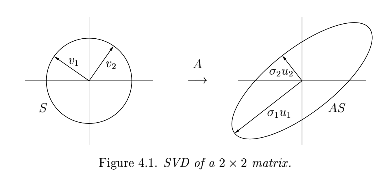
Let $S\subset \mathbb{R}^n$ be the unit sphere and take any $A\in\mathbb{R}^{m\times n}$ with $m\geq n$. For simplicity, assume for now that $\operatorname{rank}(A)=n$ (maximal in this setting). The image $A S$ is a hyperellipse in $\mathbb{R}^m$.
The $n$ singular values of $A$
These are the lengths of the $n$ principal semiaxes of $AS$: $\sigma_1, \sigma_2, \ldots, \sigma_n$. It is convenional to assume that the singular values are labeled in descending order: $\sigma_1 \geq \sigma_2 \geq \cdots \geq \sigma_n >0$.
The $n$ left singular vectors of $A$
These are the unit vectors $\{u_1,u_2,\ldots, u_n\}$ oriented in the directions of the principal semiaxes of $AS$. Their numbering matches with the corresponding singular values. The vector $\sigma_j u_j$ is the $j$-th largest principal semiaxis of $AS$.
The $n$ right singular vectors of $A$
These are the unit vectors $\{v_1,v_2,\ldots, v_n\}$ that are the preimages of the principal semiaxes of $AS$. The numbering of them is so that $A v_j = \sigma_j u_j$. Observe that each $v_j \in S$.
Don't worry about the awkward "left" vs. "right" labeling, it will be apparent below why.
Reduced SVD (or Thin SVD)
The starting point is the relation $$ A v_j = \sigma_j u_j, \qquad 1\leq j \leq n. $$
The matrix equation for this relation is $$ A V = \hat{U} \hat{\Sigma} $$ where
$V$ is the $n\times n$ matrix with orthonormal columns $V_{:,j} = v_j$, $1\leq j \leq n$.
$\hat{U}$ is the $m\times n$ matrix with orthonormal columns (recall that $m\geq n$) $\hat{U}_{:,j}=u_j$, $1\leq j \leq n$.
$\hat{\Sigma}$ is the $n\times n$ diagonal matrix $\hat{\Sigma} = \operatorname{diag}(\sigma_1,\sigma_2,\ldots,\sigma_n)$ with positive real entries (since $A$ was assumed to have full rank $n$).
Since $V$ is unitary (a square matrix), we can multiply on the right by its inverse (= its Hermitian) $V^{-1}=V^*$ to obtain $$ A = \hat{U} \hat{\Sigma} V^*. $$
This factorization of $A$ is called a reduced singular value decompotision or reduced SVD of $A$.
It looks like the following figure.
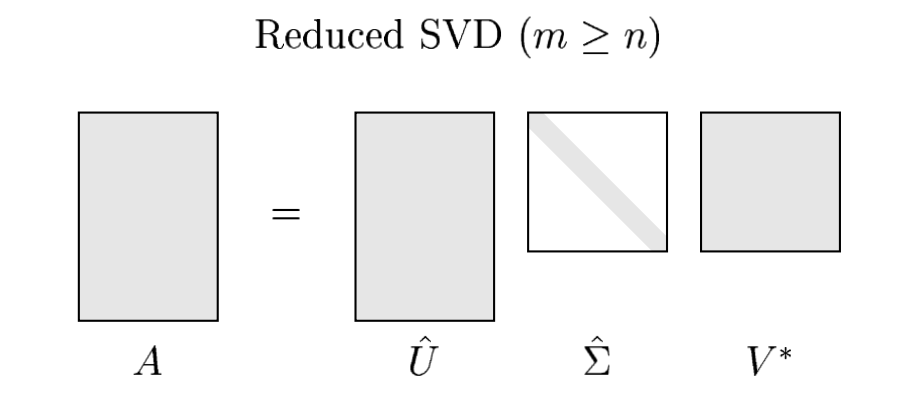
In most applications, this is the form of SVD that is used. But this is not the way the idea is formulated in the general literature. That's why we used "hats" in labeling of the matrices and called it "reduced".
The main issue is the following:
The columns of $\hat{U}$ are $n$ orthonormal vectors in $\mathbb{C}^m$. Unless $m=n$, they do not form a basis of $\mathbb{C}^m$, nor is $\hat{U}$ is a unitary matrix.
To fix this we can append $m-n$ orthonormal columns to $\hat{U}$ and extend $\hat{U}$ to an $m\times m$ unitary matrix $U$.
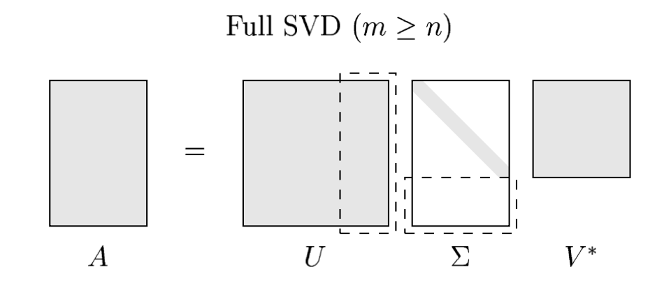
If we relace $\hat{U}$ with $U$ in SVD, we need to modify the diagonal matrix of singular values $\hat{\Sigma}$ to have compatible dimensions. It is wise to append $m-n$ zero rows $\hat{\Sigma}$ to extend it to an $m\times n$ matrix $\Sigma$. $\Sigma$ consists of the diagonal matrix $\hat{\Sigma}$ in the upper $n\times n$ block and $m-n$ zero rows in the bottom of this diagonal block.
The "full SVD" now follows:
$$ A = U \Sigma V^* $$Here $U$ is $m\times m$ and unitary, $V$ is $n\times n$ and unitary, and $\Sigma$ is $m\times n$ and diagonal with positive real entries. Schematically the full SVD looks like:
We can now let go off the full rank assumption on $A$. If $A$ has a rank deficit, all we need to do is to append $m-r$ (more compared to $m-n$) zero columns to $\hat{U}$ and so on.
Formal Definition
Let $m$ and $n$ be arbitrary --- we do not require $m\geq n$.
Given $A\in\mathbb{C}^{m\times n}$, not necessarily of full rank, a singular value decomposition (SVD) of $A$ is a factorization $$ A= U \Sigma V^* $$ where
- $U\in\mathbb{C}^{m\times m}$ is unitary,
- $V\in\mathbb{C}^{n\times n}$ is unitary,
- $\Sigma\in\mathbb{R}^{m\times n}$ is diagonal (diagonal in the generalized sense involving padded zero rows or columns if necessary).
This defintion also assumes that the diagonal entries $\sigma_j$ of $\Sigma$ are nonnegative and in nonincreasing order: $\sigma_1 \geq \sigma_2 \geq \cdots \geq \sigma_p \geq 0$, where $p=\min(m,n)$.
Note that $\Sigma$ always has the same shape as $A$.
Exercise: Reason geometrically why every matrix has an SVD using the idea of mapping the unit sphere in $\mathbb{R}^n$ via acting on it by $A$.
Full vs Thin (Reduced) SVD
The material above shows that calling a full SVD on a rectangular ($m\times n$ with $m>n$) carries unnecessary baggage.
Let $A\in\mathbb{C}^{m\times n}$ with $m>n$ (so the matrix at hand is tall and skinny) and recall the SVD
$$ A = U \Sigma V^*, $$where $U\in \mathbb{C}^{m\times m}$ is unitary, $\Sigma\in m\times n$ is diagonal, and $V\in \mathbb{C}^{n\times n}$ is unitary.
Note that $\dim(\operatorname{range}(A)) \leq n$. According to what we have explained, $$ U = [\hat{U}\quad U_2]\qquad \Sigma = \begin{bmatrix} \hat{U} \\ \mathbf{0}\end{bmatrix} $$ and here $U_2$ consists of $m-n$ columns which are a basis for the orthogonal complement of $\operatorname{range}(A)$ (assuming rank is $n$) in $\mathbb{C}^m$. But as we said above, we can modify this remainder matrix without changing $A$.
A=rand(6,3)
6×3 Matrix{Float64}:
 0.67631    0.620438  0.900084
 0.0064466  0.984052  0.238469
 0.649959   0.117057  0.498447
 0.641013   0.811401  0.922076
 0.304654   0.159673  0.795885
 0.351738   0.547861  0.242924
rank(A)
3
using LinearAlgebra
U, Σ, V = svd(A, full=true)
SVD{Float64, Float64, Matrix{Float64}, Vector{Float64}}
U factor:
6×6 Matrix{Float64}:
 -0.540951  -0.150828   -0.0214892  -0.567682   -0.595898  -0.0824892
 -0.306203   0.790787    0.149277   -0.201422    0.312361  -0.34709
 -0.300774  -0.42096    -0.532479   -0.0608112   0.515371  -0.423661
 -0.586105   0.0306636   0.0422207   0.778808   -0.213725  -0.0392116
 -0.324847  -0.34979     0.694971   -0.132166    0.447217   0.267704
 -0.272215   0.226728   -0.457115   -0.0972574   0.189863   0.787421
singular values:
3-element Vector{Float64}:
 2.363229937178218
 0.8929622879342382
 0.36638398694168145
Vt factor:
3×3 Matrix{Float64}:
 -0.479738  -0.570713  -0.666437
 -0.422947   0.815897  -0.394245
 -0.768744  -0.092733   0.632798
Verify that $U$ and $V$ are unitary:
U'*U |>display
V'*V |>display
6×6 Matrix{Float64}:
  1.0          -3.5492e-17   -3.19271e-17  …   1.49231e-16  8.05902e-17
 -3.5492e-17    1.0           8.70473e-17     -9.67623e-17  3.39866e-18
 -3.19271e-17   8.70473e-17   1.0              2.32077e-17  3.78752e-17
  7.07271e-17   7.68712e-17   1.71772e-17      9.07887e-17  1.82627e-17
  1.49231e-16  -9.67623e-17   2.32077e-17      1.0          6.67744e-17
  8.05902e-17   3.39866e-18   3.78752e-17  …   6.67744e-17  1.0
3×3 Matrix{Float64}:
 1.0           5.55112e-17   0.0
 5.55112e-17   1.0          -1.11022e-16
 0.0          -1.11022e-16   1.0
Now the thin SVD:
using LinearAlgebra
Uhat, Σhat, V = svd(A, full=false)
SVD{Float64, Float64, Matrix{Float64}, Vector{Float64}}
U factor:
6×3 Matrix{Float64}:
 -0.540951  -0.150828   -0.0214892
 -0.306203   0.790787    0.149277
 -0.300774  -0.42096    -0.532479
 -0.586105   0.0306636   0.0422207
 -0.324847  -0.34979     0.694971
 -0.272215   0.226728   -0.457115
singular values:
3-element Vector{Float64}:
 2.363229937178218
 0.8929622879342382
 0.36638398694168145
Vt factor:
3×3 Matrix{Float64}:
 -0.479738  -0.570713  -0.666437
 -0.422947   0.815897  -0.394245
 -0.768744  -0.092733   0.632798
# Compare U vs Uhat

U|>display
Uhat|>display
6×6 Matrix{Float64}:
 -0.540951  -0.150828   -0.0214892  -0.567682   -0.595898  -0.0824892
 -0.306203   0.790787    0.149277   -0.201422    0.312361  -0.34709
 -0.300774  -0.42096    -0.532479   -0.0608112   0.515371  -0.423661
 -0.586105   0.0306636   0.0422207   0.778808   -0.213725  -0.0392116
 -0.324847  -0.34979     0.694971   -0.132166    0.447217   0.267704
 -0.272215   0.226728   -0.457115   -0.0972574   0.189863   0.787421
6×3 Matrix{Float64}:
 -0.540951  -0.150828   -0.0214892
 -0.306203   0.790787    0.149277
 -0.300774  -0.42096    -0.532479
 -0.586105   0.0306636   0.0422207
 -0.324847  -0.34979     0.694971
 -0.272215   0.226728   -0.457115
The following returns the $n\times n$ ($3\times 3$) identity matrix.
Uhat'*Uhat
3×3 Matrix{Float64}:
  1.0          -3.5492e-17   -3.19271e-17
 -3.5492e-17    1.0           8.70473e-17
 -3.19271e-17   8.70473e-17   1.0
But the following does NOT return the $m\times m$ ($6\times 6$) identity matrix:
Uhat*Uhat'
6×6 Matrix{Float64}:
 0.315839    0.0431606   0.237639  0.311522   0.21355     0.122881
 0.0431606   0.741389   -0.320279  0.210018  -0.0733968   0.194411
 0.237639   -0.320279    0.551206  0.140896  -0.125104    0.229836
 0.311522    0.210018    0.140896  0.346242   0.209011    0.147199
 0.21355    -0.0733968  -0.125104  0.209011   0.710863   -0.30856
 0.122881    0.194411    0.229836  0.147199  -0.30856     0.334461
So, with the thin SVD, the columns of $\hat{U}$ are orthonormal. However, $\hat{U}$ is not a unitary matrix (it is not square).
Existence and Uniqueness
Theorem:
Every matrix $A\in\mathbb{C}^{m\times n}$ has a singular value decomposition $$ A=U\Sigma V^*. $$ and the singular values $\{\sigma_j\}$ are uniquely determined. Furthermore, if $A$ is square and the $\sigma_j$ are distinct, the left and right singular vectors are determined up to complex phases (i.e., up to complex scalar factors of modulus 1).
Proof:
Done in class.