A Course on Numerical Linear Algebra

Instructor: Deniz Bilman

Textbook: Numerical Linear Algebra, by Trefethen and Bau.

Lecture 26: Reduction to Hessenberg or Tridiagonal Form

using LinearAlgebra
A = rand(0:20, 6, 6)

6×6 Matrix{Int64}:
 14   2  18  16   8   0
  1  11   8   9  16   1
  4   0  13   8   0   4
 16  11   5  19  20  13
  5  16  19  14  18  17
 15  18  16   6  20  15

# This is what you'd get when the iterative algorithm 
# computing the Schur factorization converges
(T,Q) = schur(A);
T

6×6 Matrix{Float64}:
 65.9173   6.91374  12.9358    11.9099    -2.30041    16.867
  0.0     16.0483   -0.639618   4.87063    8.26544     0.519912
  0.0      0.0      -0.216094  12.2684     5.40949     0.550169
  0.0      0.0      -7.56057   -0.216094   7.5363     -0.393075
  0.0      0.0       0.0        0.0        0.174992  -13.2969
  0.0      0.0       0.0        0.0        0.0         8.29157

The Schur form of a matrix always exists and the eigenvalues sit at the diagonal of $T$ and stare at us.

Λ = eigvals(A)

6-element Vector{ComplexF64}:
 -0.216094247712258 - 9.630996572139273im
 -0.216094247712258 + 9.630996572139273im
 0.1749915319448782 + 0.0im
  8.291565276575604 + 0.0im
 16.048344415238855 + 0.0im
  65.91728727166523 + 0.0im

In case the eigenvalues are complex-valued, there is a way to handle the process with real arithmetic, and the resulting matrix $T$ becomes quasi-triangular, with complex eigenvalues being represented as the eigenvalues of $2\times 2$ blocks on its diagonal. This choice can be made for speed purposes.

T[3:4,3:4]|>display
a=(T[3:4,3:4])[1,1];
b=(T[3:4,3:4])[1,2];
c=(T[3:4,3:4])[2,1];
d=(T[3:4,3:4])[2,2];

2×2 Matrix{Float64}:
 -0.216094  12.2684
 -7.56057   -0.216094

b*c < 0.

true

a + 1im*sqrt(-b*c)

-0.216094247712258 + 9.630996572139274im

eigvals(T[3:4,3:4])

2-element Vector{ComplexF64}:
 -0.216094247712258 - 9.630996572139273im
 -0.216094247712258 + 9.630996572139273im

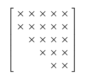
OK. But we first transform to an upper-Heisenberg matrix (all entries below the first subdiagonal are zero.). That is the first phase:

$$ A\mapsto H $$

F = hessenberg(A);

H = F.H

6×6 UpperHessenberg{Float64, Matrix{Float64}}:
  14.0     -16.179    -8.56849  -13.9849     9.78923  -4.62762
 -22.8692   42.3939   32.2153    -2.97531  -12.8806   -3.95445
    ⋅       23.3027   17.3303     2.51689  -11.8056   -0.682365
    ⋅         ⋅      -14.1685     4.40003    1.00031   0.82663
    ⋅         ⋅         ⋅        -6.97764    3.60084  -2.71927
    ⋅         ⋅         ⋅          ⋅        11.8614    8.27492

# The unitary transformation that gets us to H
Matrix(F.Q)

6×6 Matrix{Float64}:
 1.0   0.0         0.0         0.0        0.0          0.0
 0.0  -0.0437269  -0.449615    0.65065    0.508113    -0.338246
 0.0  -0.174908   -0.13215    -0.55967    0.756414     0.257975
 0.0  -0.699631    0.0906378  -0.245188  -0.103325    -0.656893
 0.0  -0.218635   -0.842596   -0.161143  -0.398657     0.239452
 0.0  -0.655904    0.249399    0.421117   0.00751394   0.574625

How does this work?

One may think of unitary triangularization via Householder reflectors. But that is not a good idea. See why for yourself: remember, we will produce $Q_1^* A Q_1$. Does that result in the desired sparsity?

What is a better idea?

Do not use a unitary matrix that acts on all the rows of $A$. Instead select a Householder reflector $Q_1^*$ that leaves the first row unchanged.

Then $Q_1^* A$ will form linear combinations of rows $2,\ldots,m$ and introduce zeros in the first column in rows $3,\ldots,m$.

Now take $Q_1$ and multiply $(Q_1^* A)$ on the right to obtain $Q_1^* A Q_1$. This will leave the first column of $Q_1^* A$ unchanged! So we will not ruin our work (on introducing zeros).

This idea is repeated to introduce zeros into subsequent columns. For example, the second Householder reflector, $Q_2$, leaves the first and second rows and columns unchanged.

After repeating this process $m-2$ times, we have a product in Hessenberg form as desided.

$$ \underbrace{Q_{m-2}^* \cdots Q_2^* Q_1^*}_{Q^*} A \underbrace{Q_1 Q_2 \cdots Q_{m-2}}_Q=H . $$

Algorithm 26.1 Householder Reduction to Hessenberg Form

• for $k=1$ to $m-2$
  • $x=A_{k+1: m, k}$
  • $v_k=\operatorname{sign}\left(x_1\right)\|x\|_2 e_1+x$
  • $v_k=v_k /\left\|v_k\right\|_2$
  • $A_{k+1: m, k: m}=A_{k+1: m, k: m}-2 v_k\left(v_k^* A_{k+1: m, k: m}\right)$
  • $A_{1: m, k+1: m}=A_{1: m, k+1: m}-2\left(A_{1: m, k+1: m} v_k\right) v_k^*$

Operation Count

$$ \text { Work for Hessenberg reduction: } \quad \sim \frac{10}{3} m^3 \text { flops. } $$

Note that $A= Q H Q$ is almost a Schur factorization! One just needs to transform the subdiagonal to $0$. Recall the example output:

H

6×6 UpperHessenberg{Float64, Matrix{Float64}}:
  14.0     -16.179    -8.56849  -13.9849     9.78923  -4.62762
 -22.8692   42.3939   32.2153    -2.97531  -12.8806   -3.95445
    ⋅       23.3027   17.3303     2.51689  -11.8056   -0.682365
    ⋅         ⋅      -14.1685     4.40003    1.00031   0.82663
    ⋅         ⋅         ⋅        -6.97764    3.60084  -2.71927
    ⋅         ⋅         ⋅          ⋅        11.8614    8.27492

The Hermitian Case: Reduction to Tridiagonal From

If $A$ is hermitian, the algorithm just described will reduce $A$ to tridiagonal form (at least, in the absence of rounding errors). This is easy to see: since $A$ is hermitian, $Q^* A Q$ is also hermitian, and any hermitian Hessenberg matrix is tridiagonal.

$$ \text { Work for tridiagonal reduction: } \quad \sim \frac{4}{3} m^3 \text { flops. } $$

# Symmetrize A and obtain B
B = A+A'

6×6 Matrix{Int64}:
 28   3  22  32  13  15
  3  22   8  20  32  19
 22   8  26  13  19  20
 32  20  13  38  34  19
 13  32  19  34  36  37
 15  19  20  19  37  30

# H for B is also Hermitian, therefore tridiagonal (banded matrix).
hessenberg(B)

Hessenberg{Float64, UpperHessenberg{Float64, Matrix{Float64}}, Matrix{Float64}, Vector{Float64}, Bool}
Q factor: 6×6 LinearAlgebra.HessenbergQ{Float64, Matrix{Float64}, Vector{Float64}, false}
H factor:
6×6 UpperHessenberg{Float64, Matrix{Float64}}:
  28.0    -43.715     4.18911e-15  -1.92664e-15   5.40675e-16  -4.4296e-15
 -43.715   92.6007  -50.2489       -1.7034e-14   -6.1369e-15   -2.55385e-15
    ⋅     -50.2489   43.1229       -6.92658       5.22226e-16   3.66116e-15
    ⋅        ⋅       -6.92658      -5.80194       6.96338       4.35548e-15
    ⋅        ⋅         ⋅            6.96338      13.778         8.95241
    ⋅        ⋅         ⋅             ⋅            8.95241       8.30033

Stability

Theorem:

Let the Hessenberg reduction $A=Q H Q^*$ of a matrix $A \in$ $\mathbb{C}^{m \times m}$ be computed by Algorithm 26.1 on a computer satisfying the axioms A and B (from Lecture 13), and let $\tilde{Q}$ and $\tilde{H}$ the computed factors (again taking $\tilde{Q}$ to be exactly unitary - see Lecture 16). Then we have

$$ \tilde{Q} \tilde{H} \tilde{Q}^*=A+\delta A, \quad \frac{\|\delta A\|}{\|A\|}=O\left(\epsilon_{\text {M}}\right) $$

for some $\delta A \in \mathbb{C}^{m \times m}$.