A Course on Numerical Linear Algebra

Instructor: Deniz Bilman

Textbook: Numerical Linear Algebra, by Trefethen and Bau.

Lecture 25: Overview of Eigenvalue Algorithms

Most of the algorithms proceed in two phases: first, a preliminary reduction from full to structured form; then, an iterative process for the final convergence.

Shortcomings of Obvious Algorithms

Let $A$ be $\mathbb{C}^{m\times m}$.

Obvious idea: Compute the coefficients of the characteristic polynomial $p_A(z)$ and do rootfinding? Forget about it.

Another idea: One can check that the sequence

$$ \frac{x}{\|x\|}, \frac{A x}{\|A x\|}, \frac{A^2 x}{\left\|A^2 x\right\|}, \frac{A^3 x}{\left\|A^3 x\right\|}, \cdots $$

converges (under certain assumptions) to an eigenvector corresponding to the largest eigenvalue of $A$ in absolute value.

Once an eigenvalue is found, one deflates and computes again and so on...

This method for finding an eigenvector is called power iteration. Although it is famous, it is not effective because it is very slow except for special matrices.

Instead of these direct ideas, the best general-purpose eigenvalue algorithms turn out to be those that compute an eigen-value revealing factorization of $A$ (the eigenvalues appear as the entries of one of the factors).

A Note on a Fundamental Difficulty

We have just recalled that finding eigenvalues of a matrix can be rephrased as finding roots of a polynomial.

More is true. Any polynomial rootfinding problem can be stated as an eigenvalue problem.

Given the monic polynomial $$ p(z)=z^m+a_{m-1} z^{m-1}+\cdots+a_1 z+a_0, $$

one can construct the companion matrix

$$ A=\begin{bmatrix} 0 & & & & & -a_0 \\ 1 & 0 & & & & -a_1 \\ & 1 & 0 & & & -a_2 \\ & & 1 & \ddots & & \vdots \\ & & & \ddots & 0 & -a_{m-2} \\ & & & & 1 & -a_{m-1} \end{bmatrix}. $$

One can show that $p(z) = (-1)^m \det(A-z \mathbb{I})$, so the roots of the polynomial $p(z)$ we are given are exactly the eigenvalues of $A$.

Here is a catch: Thanks to Abel (and Galois), we have

Theorem:

For any $m \geq 5$, there is a polynomial $p(z)$ of degree $m$ with rational coefficients that has a real root $p(r)=0$ with the property that $r$ cannot be written using any expression involving rational numbers, addition, subtraction, multiplication, division, and $k$th roots.

You see? This means that even if we could work in exact arithmetic, there could be no computer program that would produce the exact roots of an arbitrary polynomial in a finite number of steps.

By the relation above, the same is true for an eigenvalue solver. The take-away is the following:

Any eigenvalue solver must be iterative.

The goal of an eigenvalue solver is to produce sequences of numbers that converge rapidly towards eigenvalues.

Schur Factorization and Diagonalization

Most of the general-purpose eigenvalue algorithms compute the Schur factorization $A=Q T Q^*$ by transforming $A$ by a sequence of elementary unitary similarity transformations

$$ X\mapsto Q_j^* X Q_j $$

so that the product

$$ \underbrace{Q_j^* \cdots Q_2^* Q_1^*}_{Q^*} A \underbrace{Q_1 Q_2 \cdots Q_j}_Q $$

converges to an upper-triangular matrix $T$ as $j\to\infty$.

Suppose $A$ is Hermitian. Then $Q_j^* \cdots Q_2^* Q_1^* A Q_1 Q_2 \cdots Q_j$ is also Hermitian, and thus the limit of the converging sequence is both triangular and Hermitian, hence diagonal. This implies that the same algorithms that compute a unitary triangularization of a general matrix also compute a unitary diagonalization of a Hermitian matrix.

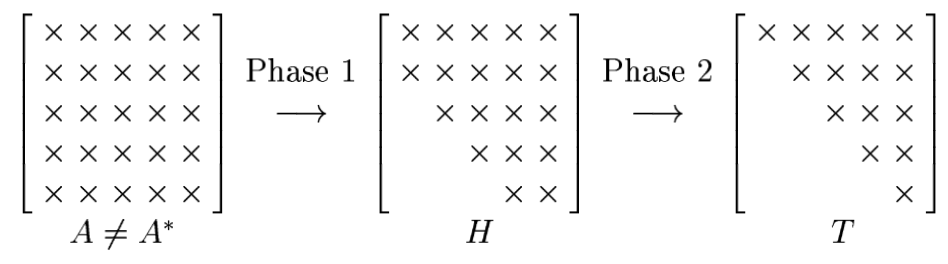
Two Phases of Eigenvalue Computations

Whether or not $A$ is hermitian, the sequence above is usually split into two phases.

In the first phase, a direct method is applied to produce an upper-Hessenberg matrix $H$. This is a matrix with zeros below the first subdiagonal.

In the second phase, an iteration is applied to generate a formally infinite sequence of Hessenberg matrices that converge to a triangular form.

Why are we doing this?

Eigenvalue algorithms are iterative. Iteration can be performed faster if the matrix has some sparsity (a structure of zeros). Getting to an upper Hessenberg matrix first bakes that structure in.