A Course on Numerical Linear Algebra
Instructor: Deniz Bilman
Textbook: Numerical Linear Algebra, by Trefethen and Bau.
Lecture 21: Pivoting
As we've seen in Lecture 20, out-of-the-box Gaussian elimination is unstable. This instability can be controlled by permuting the rows of the matrix being operated on – this is called pivoting.
Pivots
Let $X$ be the matrix we are working with at step $k$ of the Gaussian elimination.
From every entry in the submatrix $X_{k+1: m, k: m}$ is subtracted the product of a number in row $k$ and a number in column $k$, divided by $X_{k k}$
We call $X_{k k}$ the pivot.
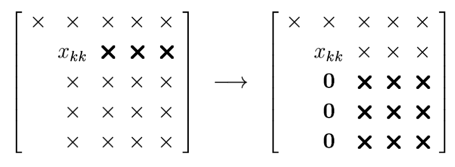
The acting $L_k$ is therefore of the form
$$ L_k=\begin{bmatrix} 1 & & & & & \\ & \ddots & & & & \\ & & 1 & & & \\ & & -\ell_{k+1, k} & 1 & & \\ & & \vdots & & \ddots & \\ & & -\ell_{m k} & & & 1 \end{bmatrix} $$with
$$ \ell_{j k}=\frac{X_{j k}}{X_{k k}} \qquad k<j \leq m. $$There is nothing special about following the diagonal. We don't have to chose the $k$th row and column in elimination at step $k$.
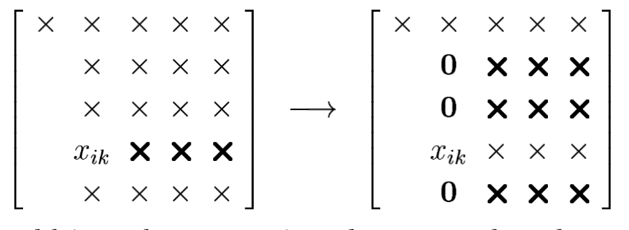
We could introduce zeros in column $k$ (we are at step $k$), by adding multiples of some row $i$ with $k<i\leq m$ to the other rows $k,k+1,\ldots,m$.
Here is an illustration with $k=2$ and $i=4$:
Similarly, we could introduce zeros in column $j$ rather than column $k$. Here is an illustration with $k=2, i=4, j=3$ :
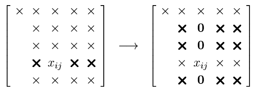
We are free to choose any entry of $X_{k: m, k: m}$ as the pivot, as long as it is nonzero.
For numerical stability, it is desirable to pivot even when $X_{k k}\neq 0$ if there is a larger element available. In practice, it is common to pick as pivot the largest number among a set of entries being considered as candidates.
This practice would complicate things if we were to keep track of the location of the pivot and implement the steps of the algorithm accordingly. So, instead, at step $$k, we permute the rows and columns of the working matrix $X$ so as to move the chosen pivot $X_{ij}$ into the $(k,k)$ position. Then, when the elimination is done, zeros are introduced into entries $k+1, \ldots, m$ of column $k$, just as in Gaussian elimination without pivoting. This interchange of rows and perhaps columns is what is usually thought of as pivoting.
One can achieve this either by actually swapping the data on the computer, or by just keeping track of permuted indices. Which approach is best depends on many factors.
Partial Pivoting
Suppose we search every entry of the submatrix $X_{k: m, k: m}$ to determine the largest. This amounts to searching $O((m-k))^2$ entries to be examined. Summing over $m$ steps, the total cost of selecting pivots alone becomes $O(m^3)$ operations, adding significantly to the cost of Gaussian elimination. This expensive strategy is called complete pivoting.
One can also find good pivots by considering a much smaller number of entries: just interchange the rows. This is called partial pivoting.
- The pivot at each step is chosen as the largest of the $m-k+1$ subdiagonal entries in column $k$.
- This incurs a total cost of only $O(m-k)$ operations for selecting the pivot at each step, hence $O(m^2)$ operations overall.
- To bring the $k$ th pivot into the $(k, k)$ position, no columns need to be permuted; it is enough to swap row $k$ with the row containing the pivot.
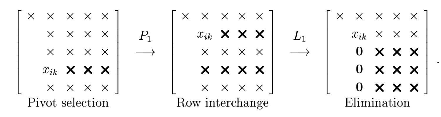
With partial pivoting, we multiply by a permutation matrix at each step before performing the row operations.
After $m-1$ steps, $A$ becomes an upper-triangular matrix $U$ :
$$ L_{m-1} P_{m-1} \cdots L_2 P_2 L_1 P_1 A=U. $$Example
Let's consider
$$ A=\begin{bmatrix} 2 & 1 & 1 & 0 \\ 4 & 3 & 3 & 1 \\ 8 & 7 & 9 & 5 \\ 6 & 7 & 9 & 8 \end{bmatrix}. $$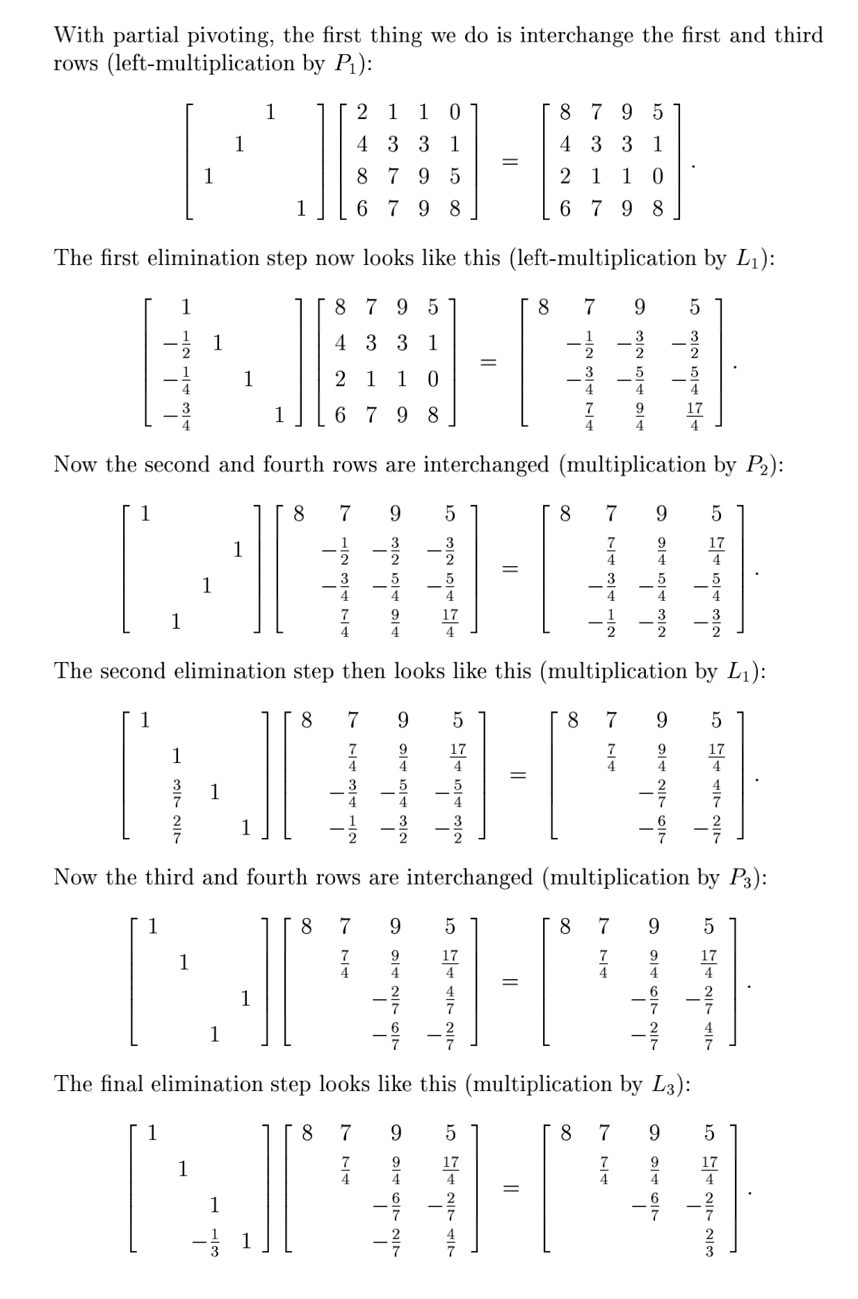
Have we computed the LU factorization of $A$? No...
A third stroke of luck is the following: We can commute the permutation matrix applied at each step with the row operation matrix.
Here is how it goes. In the example above, we have computed:
$$ L_3 P_3 L_2 P_2 L_1 P_1 A=U. $$We may write
$$ L_3 P_3 L_2 P_2 L_1 P_1=L_3^{\prime} L_2^{\prime} L_1^{\prime} P_3 P_2 P_1, $$where $L_k^{\prime}$ is equal to $L_k$ but with the subdiagonal entries permuted. To be precise, define
$$ L_3^{\prime}=L_3, \qquad L_2^{\prime}=P_3 L_2 P_3^{-1}, \qquad L_1^{\prime}=P_3 P_2 L_1 P_2^{-1} P_3^{-1} . $$Since each of these definitions applies only permutations $P_j$ with $j>k$ to $L_k$, it is easily verified that $L_k^{\prime}$ has the same structure as $L_k$. Computing the product of the matrices $L_k^{\prime}$ reveals
$$ L_3^{\prime} L_2^{\prime} L_1^{\prime} P_3 P_2 P_1=L_3\left(P_3 L_2 P_3^{-1}\right)\left(P_3 P_2 L_1 P_2^{-1} P_3^{-1}\right) P_3 P_2 P_1=L_3 P_3 L_2 P_2 L_1 P_1 $$In general for $m\times m$ matrix $A$, Gaussian elimination with partial pivoting can be written in the form
$$ \left(L_{m-1}^{\prime} \cdots L_2^{\prime} L_1^{\prime}\right)\left(P_{m-1} \cdots P_2 P_1\right) A=U, $$where $L_k^{\prime}$ is defined by
$$ L_k^{\prime}=P_{m-1} \cdots P_{k+1} L_k P_{k+1}^{-1} \cdots P_{m-1}^{-1}. $$The product of the matrices $L_k^{\prime}$ is unit lower-triangular and easily invertible by negating the subdiagonal entries, just as in Gaussian elimination without pivoting. Writing $L=\left(L_{m-1}^{\prime} \cdots L_2^{\prime} L_1^{\prime}\right)^{-1}$ and $P=P_{m-1} \cdots P_2 P_1$, we have
$$ P A=L U. $$So, we have computed the LU factorization of $PA$ rather than $A$. Indeed, Gaussian elimination with partial pivoting is equivalent to the procedure:
- Permute the rows of $A$ according to $P$
- Apply Gaussian elimination without pivoting to $P A$.
Needless to say, partial pivoting is not carried out in this way in practice, since $P$ is not known ahead of time.
Algorithm 21.1: Gaussian Elimination with Partial Pivoting
- $U=A$, $L=\mathbb{I}$, $P=\mathbb{I}$.
- for $k=1$ to $m-1$
- Select $i\geq k$ to maximize $|U_{ik}|$
- $U_{k, k: m} \leftrightarrow U_{i, k: m} \quad$ (interchange two rows)
- $\ell_{k, 1: k-1} \leftrightarrow \ell_{i, 1: k-1}$
- $P_{k,:} \leftrightarrow P_{i,:}$
- for $j=k+1$ to $m$
- $\ell_{j k}=u_{j k} / u_{k k}$
- $U_{j, k: m}=U_{j, k: m}-\ell_{j k} U_{k, k: m}$
Gaussian elimination with partial pivoting costs $\sim \frac{2}{3}m^3$ flows since the partial pivoting introduces a lower order contribution. In practice one can overwrite $U$ and $L$ to save memory. $P$ is not represented explicitly as a matrix, one uses a permutation vector (Exercise: Read about this).
using LinearAlgebra
A = [
     2.     1     1    9;
     4     3     3    1;
     8     7     9    5;
     6     7     9    8
];
display(A)
4×4 Matrix{Float64}:
 2.0  1.0  1.0  9.0
 4.0  3.0  3.0  1.0
 8.0  7.0  9.0  5.0
 6.0  7.0  9.0  8.0
# Start with permuting row 1 and row 3
P1 = Matrix{Float64}(I, 4, 4);  P1[[1 3],:] = P1[[3 1],:]
A1 = P1*A
display(A1)
L1 = Matrix{Float64}(I, 4, 4); L1[2:4,1] = -A1[2:4,1]./A1[1,1]
A1 = L1*A1
4×4 Matrix{Float64}:
 8.0  7.0  9.0  5.0
 4.0  3.0  3.0  1.0
 2.0  1.0  1.0  9.0
 6.0  7.0  9.0  8.0
4×4 Matrix{Float64}:
 8.0   7.0    9.0    5.0
 0.0  -0.5   -1.5   -1.5
 0.0  -0.75  -1.25   7.75
 0.0   1.75   2.25   4.25
# Permute row 2 and row 4
P2 = Matrix{Float64}(I, 4, 4);  P2[[2 4],:] = P2[[4 2],:]
A1 = P2*A1
display(A1)
L2 = Matrix{Float64}(I, 4, 4); L2[3:4,2] = -A1[3:4,2]./A1[2,2]
A2 = L2*A1
4×4 Matrix{Float64}:
 8.0   7.0    9.0    5.0
 0.0   1.75   2.25   4.25
 0.0  -0.75  -1.25   7.75
 0.0  -0.5   -1.5   -1.5
4×4 Matrix{Float64}:
 8.0  7.0    9.0        5.0
 0.0  1.75   2.25       4.25
 0.0  0.0   -0.285714   9.57143
 0.0  0.0   -0.857143  -0.285714
# Permute row 3 and row 4
P3 = Matrix{Float64}(I, 4, 4);  P3[[3 4],:] = P3[[4 3],:]
A2 = P3*A2
display(A2)
L3 = Matrix{Float64}(I, 4, 4); L3[4,3] = -A2[4,3]./A2[3,3]
A3 = L3*A2
4×4 Matrix{Float64}:
 8.0  7.0    9.0        5.0
 0.0  1.75   2.25       4.25
 0.0  0.0   -0.857143  -0.285714
 0.0  0.0   -0.285714   9.57143
4×4 Matrix{Float64}:
 8.0  7.0    9.0        5.0
 0.0  1.75   2.25       4.25
 0.0  0.0   -0.857143  -0.285714
 0.0  0.0    0.0        9.66667
L3*L2*L1
4×4 Matrix{Float64}:
  1.0       0.0        0.0       0.0
 -0.5       1.0        0.0       0.0
 -0.464286  0.428571   1.0       0.0
 -0.738095  0.142857  -0.333333  1.0
Note that all the subdiagonal elements have size strictly less than $1$. This will always be the case! Why?