A Course on Numerical Linear Algebra

Instructor: Deniz Bilman

Textbook: Numerical Linear Algebra, by Trefethen and Bau.

Lecture 20: Gaussian Elimination

We are back at solving a system of linear equations $Ax = b$. A more typical algorithm is the Gaussian elimination.

Gaussian elimination transforms a full linear system into an upper-triangular one by applying simple linear transformations on the left.

But the transformations are not unitary (in contrast with Householder triangularization for computing QR factorizations).

In Gaussian elimination the transformations applied are not unitary.

Let $A \in \mathbb{C}^{m \times m}$.

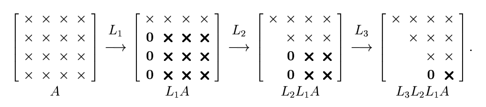
Idea: Transform $A$ into an $m\times m$ upper-triangular matrix $U$ by introducing zeros below the diagonal. Do this iteratively: first in column 1, then in column 2, and so on.

This introduction of zeros in subdiagonal similar to what Householder triangularization achieves.

But the elimination of non-zero elements is achieved by subtracting multiples of each row from subsequent rows (instead of a unitary operation as in Householder).

This is equivalent to multiplying $A$ by a sequence of lower-triangular matrices $L_k$ on the left:

$$ \underbrace{L_{m-1} \cdots L_2 L_1}_{L^{-1}} A=U . $$

Setting $L=L_1^{-1} L_2^{-1} \cdots L_{m-1}^{-1}$ gives

$$ A = LU $$

So Gaussian elimination results in an LU factorization of $A$. U is upper-triangular and L is lower-triangular.

It turns out that $L$ is unit lower-triangular: $\operatorname{diag}(L) = \mathbb{I}$.

Gram-Schmidt: $A=Q R$ by triangular orthogonalization,

Householder: $A=Q R$ by orthogonal triangularization,

Gaussian elimination: $A=L U$ by triangular triangularization.

How does this work for a general $m\times m$ matrix?

Let $X_{:,k}$ denote the $k$th column of the matrix at the beginning of step $k$ (so, $A$ has been transformed already $k-1$ times, it is no longer $A$, we just call it the matrix $X$). At step $k$, the transformation by $L_k$ involves

$$ X_{:,k}=\begin{bmatrix} X_{1 k} \\ \vdots \\ X_{k k} \\ X_{k+1, k} \\ \vdots \\ X_{m k} \end{bmatrix} \quad \xrightarrow{L_k} \quad L_k X_{:,k}=\begin{bmatrix} X_{1 k} \\ \vdots \\ X_{k k} \\ 0 \\ \vdots \\ 0 \end{bmatrix}. $$

So, we are subtracting $\ell_{jk}\times[\text{row}~k]$ from row $j$, where $\ell_{jk}$ is the multiplier

$$ \ell_{j k}=\frac{X_{j k}}{X_{k k}} \quad k<j \leq m. $$

The matrix $L_k$ is therefore of the form

$$ L_k=\begin{bmatrix} 1 & & & & & \\ & \ddots & & & & \\ & & 1 & & & \\ & & -\ell_{k+1, k} & 1 & & \\ & & \vdots & & \ddots & \\ & & -\ell_{m k} & & & 1 \end{bmatrix} $$

The diagonal is the identity and the only nonzero elements are in the subdiagonal of column $k$. This is analogous to the multiplier in step $k$ in Householder triangularization.

Strokes of luck: Remember, at the end of the day: $\underbrace{L_{m-1} \cdots L_2 L_1}_{L^{-1}} A=U$

1. $L_k$ can be inverted just by negating its subdiagonal entries.

2. The product $L$ (also lower-triangular since product of lower-triangular matrices is lower-triangular) can be formed just be collecting the entries $\ell_{jk}$ in the appropriate entries. It is like overlaying all the matrices $L_k$, or just adding their subdiagonals (since the columns with nonzero subdiagonals do not overlap).

Why do these steps work this way? (Done in class)

So we have obtained

$$ L=L_1^{-1} L_2^{-1} \cdots L_{m-1}^{-1}= \begin{bmatrix} 1 & & & & \\ \ell_{21} & 1 & & & \\ \ell_{31} & \ell_{32} & 1 & & \\ \vdots & \vdots & \ddots & \ddots & \\ \ell_{m 1} & \ell_{m 2} & \cdots & \ell_{m, m-1} & 1 \end{bmatrix}. $$

Important implementation detail: In practical Gaussian elimination, the matrices $L_k$ are never formed and multiplied explicitly. The multipliers $\ell_{j k}$ are computed and stored directly into $L$, and the transformations $L_k$ are then applied implicitly.

Algorithm 20.1: Gaussian Elimination Without Pivoting

• $U := A$ and $L:=\mathbb{I}$
• for $k=1$ to $m-1$:
  • for $j=k+1$ to $m$
    • $\ell_{j k}=U_{j k} / U_{k k}$
    • $u_{j, k: m}=U_{j, k: m}-\ell_{j k} U_{k, k: m}$

In the actual implementation, you do not need to use 3 matrices. $L$ and $U$ are not really needed. To minimize memory use on the computer, both $L$ and $U$ can be written into the same array as $A$.

Clearly, we will have issues if $U_{kk}$ is close to zero. This will be addressed later.

Operation Count

The operation count for LU factorization (Gaussian Elimination) on an $m\times m$ matrix: $\sim \frac{2}{3}m^2$ flops.

The operation count for QR factorization with Householder triangularization on an $m\times m$ matrix: $\sim \frac{4}{3}m^2$ flops.

Solving $Ax=b$ by LU Factorization

Once $A=LU$, then $Ax=b$ reduces to $LU x = b$. Thus, $Ax=b$ can be solved by solving two triangular systems:

• LU factorization requires $\sim \frac{2}{3}m^3$.
• $L y = b$ for the unknown $y$. This is forward substitution since $L$ is lower-triangular. It requires $\sim m^2$ flops.
• $U x = y$ for the unknown $x$. This is back substitution since $U$ is upper-triangular. It requires $\sim m^2$ flops.

The total work is $\sim \frac{2}{3}m^3$. This is half the total work $\sim \frac{4}{3}m^3$ required by solving $Ax=b$ via Householder triangularization.

Why is Gaussian elimination usually used rather than QR factorization to solve square systems of equations? The factor of 2 is certainly one reason. Also, Gaussian elimination has been known for centuries, whereas QR factorization of matrices did not come along until after the invention of computers.

Instability of Gaussian Elimination without Pivoting

The algorithm presented in this lecture (no pivoting) may attempt to divide by zero. That's a serious issue.

Consider

$$ A=\begin{bmatrix} 0 & 1 \\ 1 & 1\end{bmatrix}. $$

This matrix has full rank and $\kappa(A)=(3+\sqrt{5})/2\approx 2.618$ in the $2$-norm. But the Gaussian elimination fails at the first step.

using LinearAlgebra

A= [0. 1.; 1. 1.]
cond(A)

2.6180339887498953

Consider the slightly perturbed matrix now to realize a more general problem.

$$ A=\begin{bmatrix} 10^{-20} & 1 \\ 1 & 1\end{bmatrix}. $$

Now the Gaussian elimination goes through: $10^{20}\times\mathrm{1st row}$ is subtracted from the second row and we obtain the factors:

$$ L=\begin{bmatrix} 1 & 0 \\ 10^{20} & 1 \end{bmatrix}, \qquad U=\begin{bmatrix} 10^{-20} & 1 \\ 0 & 1-10^{20} \end{bmatrix} $$

A = [ 1e-20 1; 1 0 ]
L = [ 1 0 ; 1e20 1 ]
U = [ 1e-20 1; 0 -1e20 ]
display(A - L*U)

display(cond(L))

2×2 Matrix{Float64}:
 0.0  0.0
 0.0  0.0

Inf

The factos $L$ and $U$ have huge condition numbers (larger than $10^{20}$).

OK... these factors are exact though. But suppose these computations are being performed in floating point arithmetic with $\varepsilon_{\text{M}}\approx 10^{-16}$. Then the number $1-10^{20}$ in $U_{22}$ will not be represented exactly and it will be rounded to the nearest floating point. For simplicity, suppose this floating point representation is $-10^{20}$. So the floating point matrices produced would be:

$$ \tilde{L}=\begin{bmatrix} 1 & 0 \\ 10^{20} & 1 \end{bmatrix}, \qquad \tilde{U}=\begin{bmatrix} 10^{-20} & 1 \\ 0 & -10^{20} \end{bmatrix} $$

This much of rounding error seems reasonable at first sight. After all, $\|U-\tilde{U}\|/\|U\|$ is pretty small. But now compute:

$$ \tilde{L} \tilde{U} = \begin{bmatrix} 10^{-20} & 1 \\ 1 & 0 \end{bmatrix}. $$

This matrix is not at all close to $A$!!! So, if we were to solve

$$\tilde{L} \tilde{U} x = b$$

the result will be nothing like the solution to $Ax=b$. For concreteness, take $b=\begin{bmatrix} 1 \\ 0 \end{bmatrix}$. Then

$$ \tilde{L} \tilde{U} \tilde{x} = \begin{bmatrix} 1 \\ 0 \end{bmatrix} \implies \tilde{x}=\begin{bmatrix} 0 \\ 1 \end{bmatrix}, $$

whereas the correct solution is

$$ A x = \begin{bmatrix} 1 \\ 0 \end{bmatrix} \implies x\approx \begin{bmatrix} -1 \\ 1 \end{bmatrix}, $$

What is going on?

Gaussian elimination has computed the LU factorization stably: $\tilde{L}$ and $\tilde{U}$ are close to the exact factors for a matrix close to $A$ (in fact, for the matrix $A$ itself).

Yet, it has not solved $Ax=b$ stably.

The explanation is that LU factorization, though stable, \emph{was not backward stable}.

If one step of an algorithm is stable but \emph{not backward stable} for solving a subproblem, the stability of the overall calculation may be in jeopardy.

In fact, for general $m \times m$ matrices $A$, the situation is worse than this.

Gaussian elimination without pivoting is neither backward stable nor stable as a general algorithm for LU factorization.

Additionally, the triangular matrices it generates have condition numbers that may be arbitrarily greater than those of $A$ itself, leading to additional sources of instability in the forward and back substitution phases of the solution of $A x=b$.