A Course on Numerical Linear Algebra

Instructor: Deniz Bilman

Textbook: Numerical Linear Algebra, by Trefethen and Bau.

Lecture 10: Householder Triangularization

This is another approach to compute QR factorization of a matrix.

Let's remember the reduced QR factorization obtained via Gram-Schmidt iteration. The Gram-Schmidt iteration applies a succession of elementary triangular matrices $R_k$ on the right of $A$ so that the resulting matrix $Q$ has orthonormal columns:

$$ A \underbrace{R_1 R_2 \cdots R_n}_{\hat{R}^{-1}}=\hat{Q} $$

Fact: The inverse of an invertible upper-triangular matrix is upper-triangular.

Fact: The product of two upper-triangular matrices is upper-triangular.

So, the product $\hat{R} = R_n^{-1} \cdots R_2^{-1} R_1^{-1}$ is also upper-triangular and we have $A = \hat{Q}\hat{R}$ is a reduced QR factorization of $A$.

Householder

Householder algorithm constructs $Q$ as a product of unitary matrices, instead of constructing $R$. It applies a succession of elementary unitary matices $Q_k$ on the left of $A$ so that the resulting matrix is upper-triangular:

$$ \underbrace{Q_n \cdots Q_2 Q_1}_{Q^*} A=R $$

The product $Q=Q_1^* Q_2^* \cdots Q_n^*$ is unitary too, and therefore $A=Q R$ is a full QR factorization of $A$.

So the perspective is the following.

Gram-Schmidt: triangular orthogonalization,

Householder: orthogonal triangularization.

Householder Reflectors

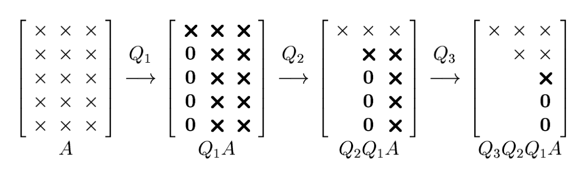
How do we construct the unitary matrices $Q_k$ to introduce zeros in the lower-triangular part of the matrix to arrive at an upper-triangular matrix?

$Q_1$ is a unitary matrix that rotates the first column of $A$ to lie on one coordinate axis.

$Q_2$ leaves the first row invariant (acts as identity), and performs a similar rotation on the vector consisting of the remaining entries of the second column of $Q_1 A$.

$Q_3$ leaves the first two rows invariant (acts as identity), and performs a similar rotation on the vector consisting of the remaining entries of the third column of $Q_2 Q_1 A$.

And so on...

The unitary matrices $Q_k$ are constructed using Householder reflectors.

Each $Q_k$ is an $m\times m$ matrix that is of the form

$$ Q_k = \begin{bmatrix} \mathbb{I}_{(k-1)\times (k-1)} & \mathbf{0} \\ \mathbf{0} & F\end{bmatrix}, $$

where $F$ is an $(m-k+1)\times (m-k+1)$ matrix that introduces zeros into the $k$th column as described above. The Householder algorithm chooses $F$ to be a particular matrix called a Householder reflector.

F acts on $x\in \mathbb{C}^{m-k+1}$ as

$$ F x = \begin{bmatrix} \|x\|_2 \\ 0 \\ 0 \\ \vdots \\ 0 \end{bmatrix} = \|x\|_2 e_1 $$

with $e_1 \in \mathbb{C}^{m-k+1}$. Note that $F^* F = \mathbb{I}$.

Let's understand the role of $F$ better. Given a vector $x$,let

$$ v = \|x\|_2 e1 - x. $$

$F$ reflects the sapce $\mathbb{C}^{m-k+1}$ across the hyperplane $H$ orthogonal to $v = \|x\|_2 e1 - x$.

When the reflector is applied, every point on one side of the hyperplane $H$ is mapped to its mirror image on the other side. In particular, $x$ is mapped to $\|x\| e_1$.

We know that for any vector $y$

$$ P y=\left(\mathbb{I}-\frac{v v^*}{v^* v}\right) y=y-\left(\frac{v^* y}{v^* v}\right)v $$

is the orthogonal projection of $y$ onto the space $H$. But to reflect $y$ across $H$, we must not stop at the point obtained by subtracting $\left(\frac{v^* y}{v^* v}\right)v$, we must subtract one more copy of that vector. Therefore, the reflection $Fy$ should be given by

$$ F y=\left(\mathbb{I}-2 \frac{v v^*}{v^* v}\right) y=y-2 \left(\frac{v^* y}{v^* v}\right)v $$

We have already seen that

$$ F = \mathbb{I} - 2 \frac{v v^*}{v^* v} $$

is a unitary matrix (hence of full rank). Note that the projector $P$ involved in the process is not full rank and it differs from $F$ just by a factor of $2$.

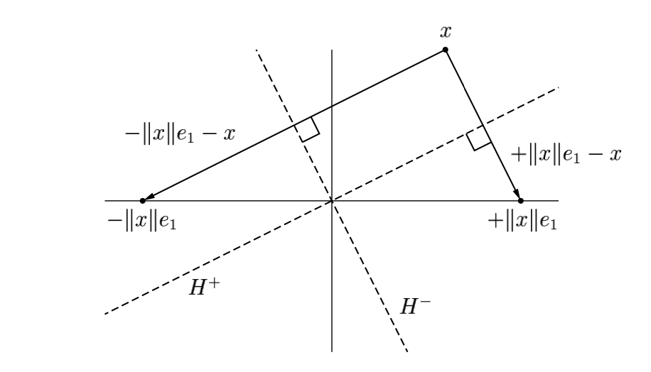
The Better of Two Reflectors

Well, we have been a bit ignorant so far. As can be seen in the Figure above, even in the real case, there exists two reflectors. The vector $x$ can be reflected to $\pm \|x\|_2 e_1$, i.e. reflected across the hyperplane $H^+$ that is the set of vectors orthogonal to $\|x\|_2 e_1 -x$ or the hyperplane $H^-$ that is the set of vectors orthogonal to $-\|x\|_2 e_1 -x$. In the complex case, there is an infinitude of such choices! The vector $x$ can be reflected to $z \|x\|_2 e_1$, where $z$ is any scalar with $|z|=1$ --- a circle of possible reflections.

For numerical stability, it is desirable to reflect $x$ to the vector $z\|x\|e_1$ that is not too close to $x$ itself, so we may choose $z=-\operatorname{sign}(x_1)$, where $x_1$ denotes the first component of $x$. So the reflection vector becomes $v=-\operatorname{sign}(x_1)\|x\|_2 e_1 -x$. Clearing the factors of $-1$, this reads

$$ v=\operatorname{sign}(x_1)\|x\|_2 e_1 + x $$

We also impose the convention that $\operatorname{sign}(x_1) = 1$ if $x_1=0$.

Why is doing this is better? In what sense it is better?

Again look at the figure (in the real case):

See, the angle between $H^+$ and the $e_1$ axis is very small compared to the angle between $H^-$ and the $e_1$ axis. The vector $v=\|x\|_2 e_1 -x$ relevant for $H^+$ is therefore smaller than $x$ or $\|x\|_2 e_1$ and the calculation of $v$ will involve subtraction of nearby quantities and will suffer from cancellation errors. If we pick the other sign, we make sure that $\|v\|_2$ is never smaller than $\|x\|_2$.

An Implementation

using LinearAlgebra

function householder_qr(A)
    m, n = size(A)
    R = copy(A)
    Q = Matrix{Float64}(I, m, m)
    
    for k in 1:min(m-1, n)
        x = R[k:m, k]
        e1 = zeros(length(x))
        e1[1] = norm(x)
        v = x + sign(x[1]) * e1
        v = v / norm(v)
        
        Hk = Matrix{Float64}(I, m, m)
        Hk[k:m, k:m] -= 2 * (v * v')
        
        R = Hk * R
        Q = Q * Hk'
    end
    
    return Q[:, 1:n], R[1:n, :]
end

# function householder_qr(A)
#     m,n = size(A)
#     Qstar = diagm(ones(m))
#     R = float(copy(A))
#     for k in 1:n
#         z = R[k:m,k]
#         w = [ -sign(z[1])*norm(z) - z[1]; -z[2:end] ]
#         nrmw = norm(w)
#         if nrmw < eps() continue; end    # skip this iteration
#         v = w / nrmw;
#         # Apply the reflection to each relevant column of A and Q
#         for j in 1:n
#             R[k:m,j] -= v*( 2*(v'*R[k:m,j]) )
#         end
#         for j in 1:m
#             Qstar[k:m,j] -= v*( 2*(v'*Qt[k:m,j]) )
#         end
#     end
#     return Qstar',triu(R)
# end

householder_qr (generic function with 1 method)

A = rand(float(1:9),8,5)
m,n = size(A)
A|>display

Q, R = householder_qr(A)

Q|>display

R|>display

8×5 Matrix{Float64}:
 4.0  6.0  5.0  2.0  5.0
 5.0  8.0  1.0  1.0  5.0
 6.0  5.0  2.0  3.0  2.0
 2.0  6.0  7.0  4.0  4.0
 7.0  1.0  6.0  6.0  5.0
 3.0  5.0  8.0  8.0  4.0
 7.0  8.0  3.0  4.0  5.0
 8.0  6.0  7.0  8.0  8.0

8×5 Matrix{Float64}:
 -0.251976  -0.270475    0.131998  -0.652293   -0.0517987
 -0.31497   -0.396449   -0.439054  -0.0386867  -0.348074
 -0.377964   0.0611347  -0.273822   0.0538295   0.73109
 -0.125988  -0.485372    0.461738  -0.267347    0.155994
 -0.440959   0.63543     0.262003  -0.295208    0.0364161
 -0.188982  -0.261212    0.555793   0.554219    0.151175
 -0.440959  -0.181552   -0.322123   0.188621    0.111356
 -0.503953   0.159321    0.142525   0.262222   -0.529862

5×5 Matrix{Float64}:
 -15.8745       -14.6146       -12.2209       -12.4098       -13.2918
   2.57988e-16   -8.56812       -2.73068       -0.424238      -2.65473
  -2.02691e-17    1.74121e-17    8.95512        6.72049        2.82679
   6.83208e-16    4.03504e-18    2.84441e-16    3.26359       -0.634911
   8.08768e-17   -2.20948e-16   -2.88384e-17    3.12092e-16   -2.80854

norm(A - Q*R)

1.608751089108294e-14